How artificial neural networks aid in mechatronic system development

Artificial neural networks are a backbone behind many data-driven artificial intelligence applications. Their popularity has grown in different domains, from speech recognition through image processing to control tasks with complex sensory inputs and multiple outputs.

In the meantime, mechatronic systems have become more complex. They now require a dedicated model-based systems development process to ensure the functional and performance design attributes.

In this blog post, we discuss how artificial neural networks aid in mechatronic systems development. We will use examples from different phases of the vehicle systems development cycle. We will also explore the applicability of various types of neural networks for a variety of engineering tasks.

Types of neural networks

Artificial neural networks (ANN) come today in many different architectures but essentially, they can be classified in three main categories:

• Feedforward neural networks (FNN), which make a direct connection between input and output data through one or more combinatorial layers
• Recurrent neural networks (RNN), which have memory of previous inputs and store data in “context nodes”
• Convolutional neural networks (CNN), which preserve spatial relations between the inputs

The mechatronic system development cycle

The mechatronic development cycle is very well established in the automotive industry. The cycle can be characterized by a few features:

• A V-process with a target cascading from system to components and verification case from components to the final system
• A double-V process representing the development cycle for the hardware as well as for the software
• An operations phase in which the data from the system in operation is fed into the next development cycle

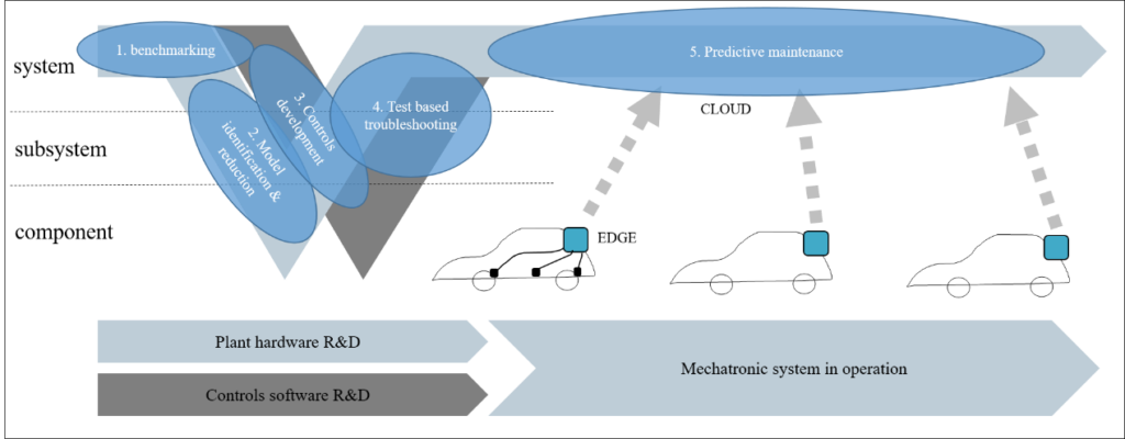
The examples used in this blog post are projected on the development lifecycle in relation to where they are applied.

Controls reverse engineering

During the benchmarking phase, many industries try to set targets for their subsystems based on a competitor analysis. Test data is typically acquired of the subsystems of a vehicle. This data is then converted into a test-based model that is assembled at system level to predict the system performance. The image below shows this process in the case of fuel economy evaluation of a vehicle.

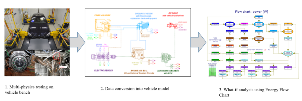
The resulting energy flow chart enables analysis of the consumption of each subsystem in the operational case that is measured. For a hybrid vehicle, there is one component that often is most difficult to identify as a test model, but often has the highest potential improvement on fuel economy performance: the supervisory control.

Using neural networks

This control determines when the different actuators need to come into play. It is often not easily converted into a model because its operation is hidden in software. This leaves the physical model only to be operated in open loop, limiting the analysis that can be done. A neural network can be used to convert the existing measurements into a controller to close the loop for the model. Performing the following steps can help to create such a controller:

• Selection of all the operational conditions to train the network
• Selecting the different sub-controller inputs and outputs based on experience
• Choosing the network architecture and size for each sub-controller
• Training of each network and cross validation with an unknown scenario
• Export of the neural network coefficients to a system simulation environment and close the loop with the plant model

Some of the steps are visualized for a controls reverse engineering of a hybrid vehicle architecture in the image below. This also includes some typical results that can be obtained.

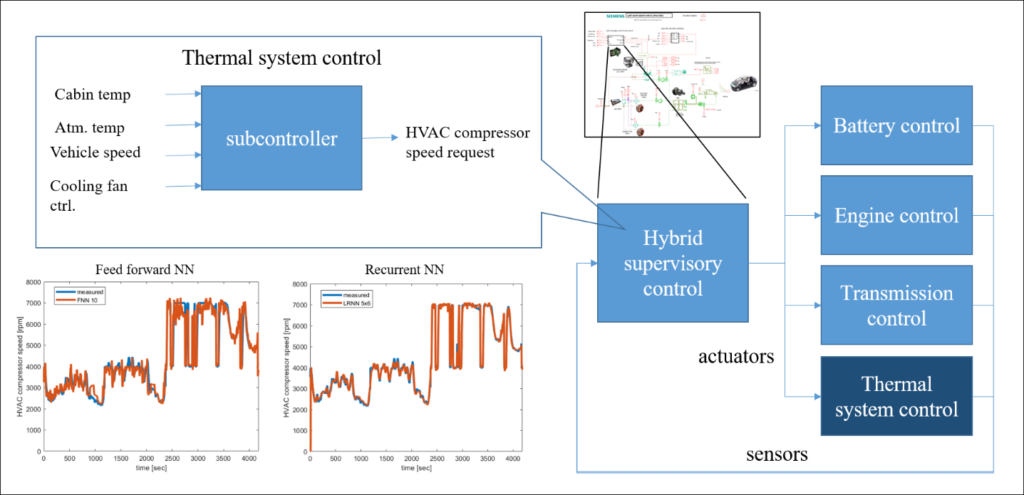
The image shows the results of the subcontroller performance using the measured operational input data of three drive cycles. The results are based on a normal feedforward network and a recurrent neural net. In both cases the correlation is good, indicating that the temporal aspects are likely unimportant for this subcontroller. When applying the complete controller to the full vehicle model, in both cases satisfactory results could be obtained.

System identification with neural networks

When building a plant model, one does not always need to have access to the full set of parameters to run it. Often a component model requires only access to the parameters for the component design engineers. However, once being designed, the system engineer only needs a surrogate model to include the physical relationships between inputs and outputs of the component into a larger system. The surrogate model can either come from test data or a more detailed model. It also must balance accuracy with calculation time.

This example shows a surrogate model of a typical engine mount. A neural network can easily be implemented into a time-domain based modeling environment since it is based on simple matrix calculations. The image below displays the application of mount stiffness identification.

In a first step, the mount stiffness is measured on a dedicated machine that allows measurement of the static and dynamic stiffnesses for different amplitudes. Converting this into a time-domain modeling environment is not straightforward. Typically an equivalent modeling approach is used based on multiple mass-spring-damper elements.

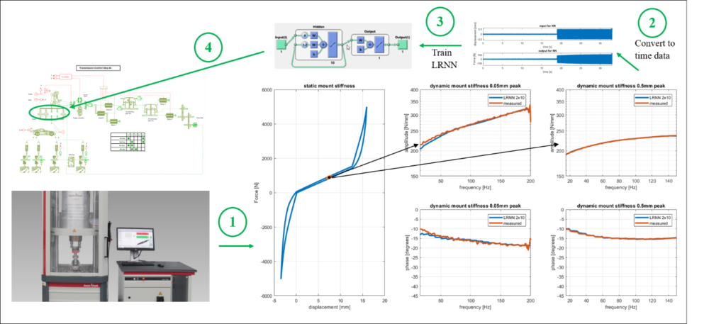
With a neural network, the dynamic stiffness curves in frequency domain can be converted into one set of training time data (upper right). In this example, the time data is fed into a layered recurrent net with 10 hidden layer neurons and two delays. The result of the trained network is validated again in frequency domain (red curve for the two different excitation amplitudes) and gives excellent correlation with the measured data.

Afterwards this neural network can be combined with the static curve. This is done by placing both models in parallel to obtain the total stiffness and implemented in a vehicle model (upper left).

Virtual sensors for predictive maintenance

Failures of bearings are caused primarily by built-up wear or damage in the bearing of a wind turbine. Offshore wind turbines are difficult to access, therefore the predictive maintenance is an important aspect of limiting the maintenance costs. In this application the bearing is modeled as a simple source of vibrations, caused by defects in the bearings. The vibrations can be measured by operational sensors in the real wind turbine. To improve the realism of the signals, different manipulations are done to the ideal time signals coming from the model:

• Addition of measurement noise
• Gaussian broadening and introduction of half-normal distribution to introduce the effect of slippage from the roller defect

These time signals could be fed to an RNN to find the relationships between the signature of the signal and the status of the defect. To help the neural network find the relationship more easily, an additional preprocessing is done based on the knowledge of the recurrence of the vibration. The postprocessing that is done to facilitate the neural network in finding the relationship are the following two steps:

• Synchronous averaging at expected defect periods
• Averaging to improve the signal-to-noise ratio

RNN or CNN?

This will result in time-invariant data that can be used to train a CNN rather than an RNN. The complete sensor processing to create the data for the neural network to be trained on is shown in the image below.

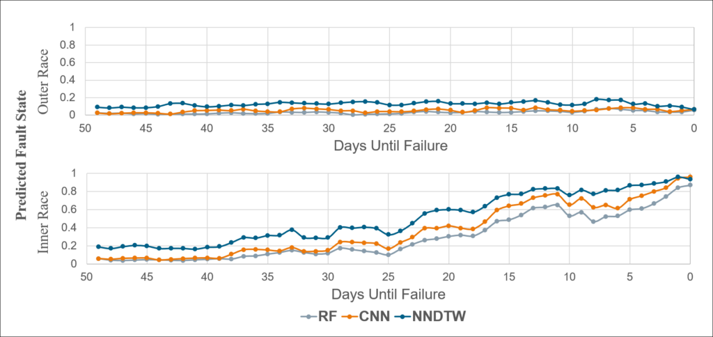
The CNN is chosen as the neural network architecture for this learning because the proximity relationship of the samples in the time-averaged signal are of importance. The CNN is used in a regression context where a value is given between fully nominal (0) or fully faulty (1). This allows the network to predict the time to failure if enough knowledge is available between the gravity of the defect and the risk of failure.

The image below shows the result of the constant monitoring during 50 days until failure using a trained CNN with only simulation data for a bearing inner ring as well as outer ring failure.

Assisting the analyst

A system analyst is a person that analyses complex data. He or she uses past experience to interpret the data and understand the problem. The analysis can be linked to test data as well as simulation data.

In this example, we will describe the use of a neural network for understanding the contributors to a noise peak.

Noise, vibration, and harshness

Noise, vibration and harshness (NVH) is an important attribute of the vehicle. It is very difficult to frontload NVH issues into the simulation-based development of the vehicle. Typically, during the first prototype stage, the road-induced and engine-induced low frequency NVH issues become visible.

NVH test engineers use methodologies like transfer path analysis (TPA) or acoustic source quantification (ASQ) to separate the noise problem into its contributing paths and afterwards focus on the major contributing paths with effective countermeasures.

The methodology of TPA is however a time-consuming activity that can be separated into two major components:

• In the first step the paths are instrumented with sensors and operational data acquired on the full system.
• In the second step, the active system (driveline and/or suspension) is removed. The contributions from unity loads at each path to the interior noise are quantified using dedicated excitation techniques.

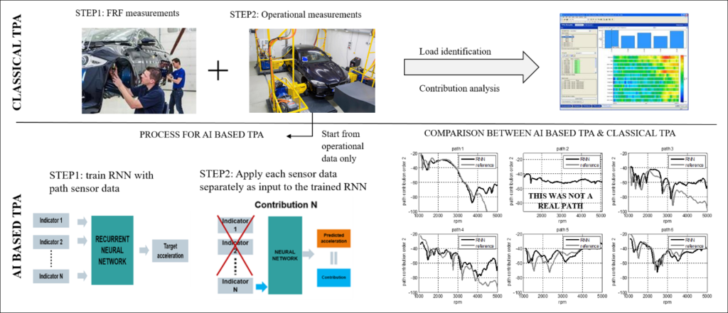
Even in this context of test-based troubleshooting, neural networks have proven to be helpful in giving the NVH engineer useful countermeasures even faster. In this approach, only the potentially contributing paths need to be instrumented for which only operational conditions need to be acquired.

During a first phase, a layered recurrent neural network is trained based on the path sensors as inputs and the noise as output. In a second phase, the trained neural network is fed with each sensor individually to be able to calculate the contributions of each path. The image below shows the results of the neural network-based approach versus the result of a classical TPA approach. In both cases the major paths are identical while the neural network-based approach can be realized in a fraction of the total time needed for the full TPA approach.

Conclusion

For mechatronic system development, artificial intelligence is finding many applications. Results that were obtained only in the last two years indicate that the potential today is unlimited. Machine learning has been applied successfully in the past for speech and image recognition; today it can be used for much more. The major advantage of neural networks within the machine learning field is the fact that their training can be tuned for each application case based on the knowledge of the application builder.

In the above examples, neural networks were successfully applied for system identification, preventative maintenance and expert analysis. These examples are not exhaustive, and many more applications of neural networks will appear in the years to come. Some major future developments we expect is the capability to derive physical models from data or the consolidation of expert knowledge into an artificial expert. Engineers can use these insights to propose design changes based on CAE analysis or even based only on the requirements of the system to be designed.

Watch our webinar “Discover the power of deploying neural networks and its impact on systems engineering” to learn more.

To get in touch with Simcenter Engineering, email us at engineeringservices.sisw@siemens.com.