The art of modelling using CFD. Part VI – Peripheral Boundary Conditions
This final blog in this series focuses on what is sometimes the most ethereal of CFD modelling arts, where and how to define your peripheral boundary conditions. A fancy phrase but in reality no more than deciding where the interface is between what you model and what you don’t. Heat is contemptuous of such divisions, it will spread out from it’s source and keep on spreading via convection, conduction and radiation until it heats up (albeit only slightly) the earth’s atmosphere. From a pragmatic perspective you can’t model the entire earth just to find an active IC’s junction temperature. You have to truncate your model somewhere and somehow.
The term ‘boundary condition’ is well used and understood when one talks of solving PDEs (partial differential equations). When applied to a 3D solution of the PDEs governing fluid flow and heat transfer (the Navier Stokes equations) the term historically applied to the outer edges of the computational domain, the volume of space in which you predicted the fluid flow. The earliest CFD models had an uninterrupted volume of fluid with solid, or well defined flow, conditions on the peripheral faces of that volume. Today, boundary condition (BC) as a phrase is used to describe a much wider range of inputs to a model, e.g. power dissipations, internal geometries etc. For now let’s use the word peripheral to focus on just those conditions that cement the interface between the volume of space you are modelling and the volume of space that you are not.
“Words offer the means to meaning” (good film, 5 fictional credits to the first person to comment as to which film, if you Google it you’re just cheating yourself, that’s what I tell my kids anyway). ‘Level’ is another word that is often used to define the type of electronics cooling simulation performed (and other types simulations as well, word re-use here can have some disastrous effects, what a thermal engineer considers a system level model really isn’t what an EE would consider). From a thermal perspective:
- Wafer level, what goes on in a silicon die
- Package level, what goes on in the packaging arond the die
- Board level, considering many components sitting on a board
- System level, the PCB(s) + chassis/box + fans + PSUs …
- Room level, considering the product operating in its final destination as in a Data Center
If you are doing simulation at any level you have to define peripheral BCs that link it to the level(s) above. Heat and fluid need to know how they enter or leave the model from or to that which you are not modelling.
Take a wafer level simulation. You are modelling a die in detail, maybe a series of stacked die to determine optimal placement fo TSVs. How do you represent the thermal effects that the unmodelled package has on the behaviour of heat in the silicon? Whether the package has a heat slug, whether the die abuts a DAP, whether there will be a heatsink on the package, all these things will affect the thermal behaviour within the die, all these conditions outside your model will have to be prescribed on the periphery of your wafer level model. For such conduction type models you would set temperatures and heat transfer coefficients on the sides of your silicon. Temperature is just that, heat transfer coefficient is a measure of how effectively heat can pass through that peripheral portion of your model. The two together prescribe the effects of the package.
Such decisions, such prescriptions, have to be made at any level of modelling. For board level you need to define how the air moves over the board. For a system level you have to set the temperature of the air coming into your box. This all begs the question where do you get such information from?
Answer 1: set these BCs based on ‘worst case’ operating environments. Doing this will enable you to verify if your package, board, room etc. will be thermally viable in the extreme
Answer 2: import such BCs from existing models of the adjacent levels. FloTHERM excels at this with a feature called ‘zoom-in’:
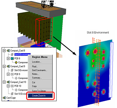
e.g. getting actual operating conditions from a system level model to impose them on a board level model. Zoom-in again from board level down to package level. Such automation leads to far more accurate simulation at any level at literally a press of a button (sorry, rather selection from a pop-up menu).
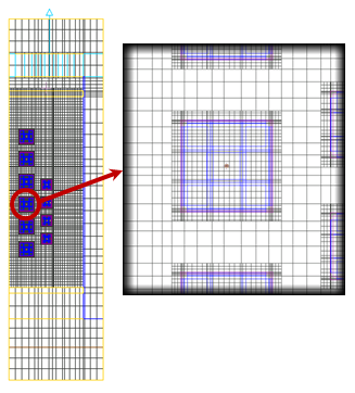
 Computational limitations and data availability have and will always continue to limit the option of combining levels together. I’m not envisioning that the world model will ever be a reality but there are methods to alleviate the computational overhead of say having detailed models of packages sitting inside a system level model. FloTHERM’s ‘localized grid’ capability started making that a reality nearly a decade ago:
Combining adjacent levels into a single model alleviates the time and effort needed to pass BCs around using zoom-in (and zoom-out). Gathering all the required information together into a single model is just as challenging though. In the glorious future all vendors will supply numerical thermal models of all of their parts, model building in CAD and CAE will be simply be a question of drag+drop, plug and play. Until that time features that improve the effectiveness of the setting of peripheral BCs will aid in the art of this aspect of CFD modelling.
21st June 2010, Ross-on-Wye